## List pacakges used in the script
packages <- c("rscopus", "RefManageR", "tidyverse","brio",
              "stringr", "bibtex", "glue", "here", "litsearchr",
              "revtools", "remotes", "igraph", "remotes",
              "PRISMAstatement", "synthesisr")

## Load packages and install them if needed
for (package in packages) {
  if (!require(package, character.only = TRUE)) {
    if (package == "litsearchr") remotes::install_github("elizagrames/litsearchr", ref="main")
    else install.packages(package)
  }
}Companion code for section 2: Search strategy & selection of references
Let us first install and load the packages we will need.
We also need to organize our repository
dir.create("raw-data") #for raw data
dir.create("processed-data") #for the unique references
dir.create("output")
1 Retrieving references from Scopus
Set your API key - if you do not have one, please go to the Elsevier Developer Portal to apply for one with your institutional credentials.
Once you have your key (i.e. a long string of digits and characters), replace Your_scopus_api_key by the key value, and add quotes, for instance: options(elsevier_api_key = “my8personal4key”)
options(elsevier_api_key = Your_scopus_api_key)Set your research query:
query <- "( ( ( TITLE ( govern* OR state OR decision-making OR policy-making OR stakeholder OR participat* ) ) AND ( TITLE-ABS-KEY ( impact OR outcome OR result OR differentiation OR consequence OR change OR transformation OR role ) ) ) OR ( TITLE-ABS-KEY ( governance W/0 ( mode OR model OR process ) ) ) ) AND
          ( TITLE-ABS-KEY ( effect OR caus* OR explain* OR influence OR affect OR mechanism OR restrict OR create OR impact OR drive OR role OR transform* OR relation* OR led OR improve OR interven* OR respon* ) ) AND
          ( TITLE-ABS-KEY ( urban OR neighborhood OR city OR residential OR regional OR housing ) W/0 ( development OR redevelopment OR regeneration OR restructuring OR revitalization OR construction OR governance ) ) "
Query scopus if you get the api key. Note that you can modify the max_count for each searching:
if (have_api_key()) {
  res <- scopus_search(query = query, max_count = 200, count = 10, view = "COMPLETE")
  search_results <- gen_entries_to_df(res$entries)
}
The query list is: list(query = "( ( ( TITLE ( govern* OR state OR decision-making OR policy-making OR stakeholder OR participat* ) ) AND ( TITLE-ABS-KEY ( impact OR outcome OR result OR differentiation OR consequence OR change OR transformation OR role ) ) ) OR ( TITLE-ABS-KEY ( governance W/0 ( mode OR model OR process ) ) ) ) AND \n ( TITLE-ABS-KEY ( effect OR caus* OR explain* OR influence OR affect OR mechanism OR restrict OR create OR impact OR drive OR role OR transform* OR relation* OR led OR improve OR interven* OR respon* ) ) AND \n ( TITLE-ABS-KEY ( urban OR neighborhood OR city OR residential OR regional OR housing ) W/0 ( development OR redevelopment OR regeneration OR restructuring OR revitalization OR construction OR governance ) ) ",
count = 10, start = 0, view = "COMPLETE")
$query
[1] "( ( ( TITLE ( govern* OR state OR decision-making OR policy-making OR stakeholder OR participat* ) ) AND ( TITLE-ABS-KEY ( impact OR outcome OR result OR differentiation OR consequence OR change OR transformation OR role ) ) ) OR ( TITLE-ABS-KEY ( governance W/0 ( mode OR model OR process ) ) ) ) AND \n ( TITLE-ABS-KEY ( effect OR caus* OR explain* OR influence OR affect OR mechanism OR restrict OR create OR impact OR drive OR role OR transform* OR relation* OR led OR improve OR interven* OR respon* ) ) AND \n ( TITLE-ABS-KEY ( urban OR neighborhood OR city OR residential OR regional OR housing ) W/0 ( development OR redevelopment OR regeneration OR restructuring OR revitalization OR construction OR governance ) ) "
$count
[1] 10
$start
[1] 0
$view
[1] "COMPLETE"
Response [https://api.elsevier.com/content/search/scopus?query=%28%20%28%20%28%20TITLE%20%28%20govern%2A%20OR%20state%20OR%20decision-making%20OR%20policy-making%20OR%20stakeholder%20OR%20participat%2A%20%29%20%29%20AND%20%28%20TITLE-ABS-KEY%20%28%20impact%20OR%20outcome%20OR%20result%20OR%20differentiation%20OR%20consequence%20OR%20change%20OR%20transformation%20OR%20role%20%29%20%29%20%29%20OR%20%28%20TITLE-ABS-KEY%20%28%20governance%20W%2F0%20%28%20mode%20OR%20model%20OR%20process%20%29%20%29%20%29%20%29%20AND%20%0A%20%20%20%20%20%20%20%20%20%20%28%20TITLE-ABS-KEY%20%28%20effect%20OR%20caus%2A%20OR%20explain%2A%20OR%20influence%20OR%20affect%20OR%20mechanism%20OR%20restrict%20OR%20create%20OR%20impact%20OR%20drive%20OR%20role%20OR%20transform%2A%20OR%20relation%2A%20OR%20led%20OR%20improve%20OR%20interven%2A%20OR%20respon%2A%20%29%20%29%20AND%20%0A%20%20%20%20%20%20%20%20%20%20%28%20TITLE-ABS-KEY%20%28%20urban%20OR%20neighborhood%20OR%20city%20OR%20residential%20OR%20regional%20OR%20housing%20%29%20W%2F0%20%28%20development%20OR%20redevelopment%20OR%20regeneration%20OR%20restructuring%20OR%20revitalization%20OR%20construction%20OR%20governance%20%29%20%29%20&count=10&start=0&view=COMPLETE]
Date: 2024-05-21 07:08
Status: 200
Content-Type: application/json;charset=UTF-8
Size: 57 kBTotal Entries are 4983Maximum Count is 20020 runs need to be sent with current count
  |
  |                                                                      |   0%
  |
  |====                                                                  |   6%
  |
  |========                                                              |  11%
  |
  |============                                                          |  17%
  |
  |================                                                      |  22%
  |
  |===================                                                   |  28%
  |
  |=======================                                               |  33%
  |
  |===========================                                           |  39%
  |
  |===============================                                       |  44%
  |
  |===================================                                   |  50%
  |
  |=======================================                               |  56%
  |
  |===========================================                           |  61%
  |
  |===============================================                       |  67%
  |
  |===================================================                   |  72%
  |
  |======================================================                |  78%
  |
  |==========================================================            |  83%
  |
  |==============================================================        |  89%
  |
  |==================================================================    |  94%
  |
  |======================================================================| 100%
Number of Output Entries are 200Create an empty list to store search results
ids <- search_results$df$pii
search_results_list <- list()
for (id in ids) {
  search_results_list[[id]] <- search_results$df
}
Convert the list to a data frame
results_df <- do.call(rbind, search_results$df)
transposed_results_df <- t(results_df)
dim(transposed_results_df)
[1] 200 36Add filter to keep only articles”
articles_df <- as_tibble(transposed_results_df) |>
  filter(subtype == "ar")
dim(articles_df)
[1] 176 36What does it look like?
head(articles_df)# A tibble: 6 × 36
`@_fa` `prism:url` `dc:identifier` eid `dc:title` `dc:creator`
<chr> <chr> <chr> <chr> <chr> <chr>
1 true https://api.elsevier.com… SCOPUS_ID:8519… 2-s2… Decomposi… Wu Y.
2 true https://api.elsevier.com… SCOPUS_ID:8518… 2-s2… Explainin… Karampouria…
3 true https://api.elsevier.com… SCOPUS_ID:8518… 2-s2… De-border… Zapata-Barr…
4 true https://api.elsevier.com… SCOPUS_ID:8519… 2-s2… Artificia… Bibri S.E.
5 true https://api.elsevier.com… SCOPUS_ID:8519… 2-s2… Decipheri… Abedin J.
6 true https://api.elsevier.com… SCOPUS_ID:8519… 2-s2… Blockchai… Zhu X.
# ℹ 30 more variables: `prism:publicationName` <chr>, `prism:eIssn` <chr>,
# `prism:volume` <chr>, `prism:issueIdentifier` <chr>,
# `prism:coverDate` <chr>, `prism:coverDisplayDate` <chr>, `prism:doi` <chr>,
# `dc:description` <chr>, `citedby-count` <chr>,
# `prism:aggregationType` <chr>, subtype <chr>, subtypeDescription <chr>,
# `author-count.@limit` <chr>, `author-count.@total` <chr>,
# `author-count.$` <chr>, `article-number` <chr>, `source-id` <chr>, …Write the details to a CSV file
write.csv(articles_df, here("processed-data", "scopus_api_results.csv"), row.names = FALSE)Export a into a .bib file
df <- read.csv(here("processed-data", "scopus_api_results.csv"))
for (i in 1:nrow(df)) {
  df$authkeywords[i] <- paste(unlist(strsplit(df$authkeywords[i], "\\s*\\|\\s*")), collapse = ", ")
}

data <- data.frame(
  Author = df$dc.creator,
  Title = df$dc.title,
  Year = sub(".*\\s(\\d{4})$", "\\1", df$prism.coverDisplayDate),
  Journal = df$prism.publicationName,
  Volume = df$prism.volume,
  Number = df$article.number,
  Pages = df$prism.pageRange,
  DOI = df$prism.doi,
  Keyword = df$authkeywords
)
Create a list of BibEntry objects
# Format the Keywords field
bib_entries <- lapply(1:nrow(data), function(i) {
  BibEntry(
    bibtype = "Article",        # Add the bibtype argument
    key = paste0(substr(data$Author[i], 1, 1), data$Year[i]),
    author = data$Author[i],    # Add author field
    title = data$Title[i],      # Add title field
    year = data$Year[i],        # Add year field
    journal = data$Journal[i],  # Add journal field
    volume = data$Volume[i],    # Add volume field
    number = data$Number[i],    # Add number field
    pages = data$Pages[i],      # Add pages field
    doi = data$DOI[i],         # Add DOI field
    url = data$Keyword[i]      # Add Keyword field (because BibEntry function does not provide keyword indicator, use url for keywords as an example.)
  )
})
Convert each BibEntry object to BibTeX format individually
bib_texts <- lapply(bib_entries, toBibtex)Combine the BibTeX texts into a single character vector
bib_text <- unlist(bib_texts, use.names = FALSE)Write BibTeX file
writeLines(bib_text, here("processed-data","scopus_references.bib"))2 Combining tables, deduplicating references and summarising the results
Although a dedicated package exist to retrieve references from the Web of Science API (wosr), we have not been able to make it work. Instead, we used the web interface of the [Web of Science](https://www.webofscience.com/wos/woscc/summary/82f1ef9f-d361-4455-a556-cc37014e5f7a-de2281b0/relevance/1] (through our institutional access) to run the same query:
( ( ( TI= ( govern* OR state OR decision-making OR policy-making OR participat* OR stakeholder ) ) AND ( TS= ( impact OR outcome OR performance OR result OR differentiation OR consequence OR change OR transformation OR role ) ) ) OR ( TS= ( governance NEAR/0 ( mode OR model OR role OR process )) ) ) AND (TS= ( effect OR caus* OR explain* OR influence OR affect OR mechanism OR restrict OR create OR impact OR drive OR role OR transform* OR relation* OR led OR improve OR interven* OR respon* ) ) AND ( TS= (( urban OR neighborhood OR city OR residential OR regional OR housing ) NEAR/0 (development OR redevelopment OR renewal OR regeneration OR restructuring OR revitalization OR governance ) ) )
We then selected the articles written in English from the results and obtained 3180 results as of 11 April 2024. We downloaded the first 200 records in .bib format for this example: wos_reference.bib, and saved them in the raw-data folder of our project. Indeed, we want to show that this code can combine bibliographic data from different queries and or different databases.
wos_data <- synthesisr::read_refs(here("raw-data", "wos_reference.bib"))
scopus_data <- synthesisr::read_refs(here("processed-data", "scopus_references.bib"))

# Remember we stored keywords into the url field, let's rename it now:
scopus_data$keywords <- scopus_data$url
Save variable names of dataframes is object
unique_vars_scopus <- colnames(scopus_data)
 unique_vars_wos <- colnames(wos_data)
Identify which columns the scopus and wos dataframes have in common
common_vars <- intersect(unique_vars_scopus, unique_vars_wos)
print(common_vars)
[1] "type" "author" "title" "year" "journal" "volume"
[7] "number" "doi" "pages" "keywords"Identify which columns are unique for the scopus and wos references
unique_vars_only_scopus <- setdiff(unique_vars_scopus, unique_vars_wos)
print(unique_vars_only_scopus)
[1] "url"unique_vars_only_wos <- setdiff(unique_vars_wos, unique_vars_scopus)
print(unique_vars_only_wos) [1] "month" "abstract"
[3] "publisher" "address"
[5] "language" "affiliation"
[7] "article_number" "issn"
[9] "eissn" "keywords_plus"
[11] "research_areas" "web_of_science_categories"
[13] "author_email" "affiliations"
[15] "researcherid_numbers" "orcid_numbers"
[17] "funding_acknowledgement" "funding_text"
[19] "cited_references" "number_of_cited_references"
[21] "times_cited" "usage_count_last_180_days"
[23] "usage_count_since_2013" "journal_iso"
[25] "doc_delivery_number" "web_of_science_index"
[27] "unique_id" "da"
[29] "oa" "earlyaccessdate"
[31] "note" "organization"
[33] "book_author" "booktitle"
[35] "series" "isbn"
[37] "editor" Select only the variables that appear in both dataframes and the ones you deem relevant. In our case, we select: author, type, title, year, volume, number, pages, doi, keywords
selected_vars <- c(
 # "label",
  "author",  "title", "year", "journal",
  "volume", "number", "pages", "doi", "keywords")

scopus_selection <- scopus_data %>%
  dplyr::select(all_of(selected_vars))

wos_selection <- wos_data %>%
  dplyr::select(all_of(selected_vars))
Now lets check the number of variables (columns) in our dataframes
ncol(scopus_selection)[1] 9ncol(wos_selection)[1] 9now lets combine the wos dataframe with the scopus dataframe
all_references <- rbind(wos_selection, scopus_selection)3 Locate and extract unique references
In order to be able to identify if there are duplicates in our all_references dataframe and examine summary statistics of the references-dataset, we need to make sure that variables in the scopus and wos dataframes are represented in a similar way. Sometimes variables differ too much, such that comparison even after alteration becomes difficult (i.e. in our example the variable “author”). However, for others we we can remove all punctuations and capital letters in order to make the variable structure of the wos refences and scopus refences more similar.
Lets see how we can do that.
First create function called preprocess which removes all capital letters and punctuations
preprocess <- function(text) {
  text <- tolower(text) #all characters are transformed to lower-case
  text <- gsub("[[:punct:]]", "", text) #all punctuations are removed from the characters
  return(text)
}
Now lets apply this function on relevant variables in our all_references dataframe
all_references$journal <- sapply(all_references$journal, preprocess)
all_references$title <- sapply(all_references$title, preprocess)
all_references$author <- sapply(all_references$author, preprocess)
Examine the scopus_selection dataframe
view(all_references)as you can see, all the capital and punctuations are removed from the assigned variables
check_duplicates <- revtools::find_duplicates(all_references, match_variable = "doi")
all_unique_references <- extract_unique_references(all_references, matches = check_duplicates)
Compare the total number of references to the total number of unique references
#count the number of rows in the all_references dataframe
nrow(all_references)
[1] 376#do the same for the references_unique dataframe
nrow(all_unique_references)[1] 245Something else we might want to consider, is if our literature search also identified one or more key articles that we know should be in the SLR. So, lets take a target article. In our case, the author of this specific literature review stated that (Van Marissing et al., 2006) and (Wu & Zhang, 2022) should be considered as a target references. So let’s examine, if they are included in our all_unique_references dataframe. We do this copying doi from the target references and identifying if this doi is present in the all_unique_references dataframe
#Read target papers's bib file and extract doi information
target_references <- synthesisr::read_refs(here("raw-data", "targetPapers.bib"))

# Let's test whether they are present or not our reference list
 target_references$doi %in% all_unique_references$doi
[1] FALSE FALSEThe outcome (FALSE and FALSE) means that none of our target references is included in our all_unique_references dataframe. We should therefore modify our query so as to include them in the results. Please note that for the sake of simplicity and speed, we have restricted our search to 200 articles in each database, which is why it is most likely that we did not identify the target references in this particular example.
4 Summarise references:
Distribution of publication years
all_unique_references$year <- as.numeric(all_unique_references$year)

ggplot(all_unique_references) +
  geom_histogram(aes(x=year), fill = "orange")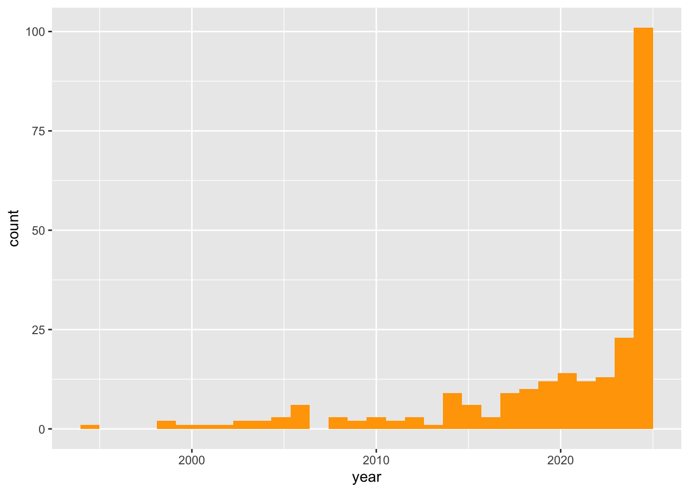
Top 10 journals publishing on topic:
all_unique_references$journal <- as.factor(all_unique_references$journal)
head(summary(all_unique_references$journal),10)
urban studies urban affairs review
9 6
journal of urban affairs urban research practice
4 4
cities land
3 3
professional geographer regional studies
3 3
sustainability sustainability switzerland
3 3 Export combined set of unique references into a .bib file:
unique_data <- data.frame(
    Author = all_unique_references$author,
  Title = all_unique_references$title,
  Year = all_unique_references$year,
  Journal = ifelse(is.na(all_unique_references$journal),
                     "Unknown",all_unique_references$journal),
  Volume = all_unique_references$volume,
  Number = all_unique_references$number,
  Pages = all_unique_references$pages,
  DOI = all_unique_references$doi,
  Keywords = all_unique_references$keywords
)

# Format the Keywords field
unique_bib_entries <- lapply(1:nrow(unique_data)
                             , function(i) {
  BibEntry(
    bibtype = "Article",        # Add the bibtype argument
    key = i,
    author = unique_data$Author[i],    # Add author field
    title = unique_data$Title[i],      # Add title field
    year = unique_data$Year[i],        # Add year field
    journal = unique_data$Journal[i],  # Add journal field
    volume = unique_data$Volume[i],    # Add volume field
    number = unique_data$Number[i],    # Add number field
    pages = unique_data$Pages[i],      # Add pages field
    doi = unique_data$DOI[i],         # Add DOI field
    url = unique_data$Keywords[i]
    )
})

unique_bib_texts <- lapply(unique_bib_entries, toBibtex)
unique_bib_text <- unlist(unique_bib_texts, use.names = FALSE)

dir.create("processed-data/unique_refs")
Warning in dir.create("processed-data/unique_refs"):
'processed-data/unique_refs' already existswriteLines(unique_bib_text, here("processed-data","unique_refs","all_unique_references.bib"))5 Suggesting new keywords
NB: Parts of this section were adapted from the litsearchr package documentation available here
Import .bib or .ris database
refs <- litsearchr::import_results(here("processed-data", "unique_refs"))Reading file /Users/ccottineau/GitHub/SLRbanism/processed-data/unique_refs/all_unique_references.bib ... doneIdentify frequent terms
raked_terms <- extract_terms(text = refs,
                             method = "fakerake",
                             min_freq=2,
                             min_n=2)
Identify frequent keywords tagged by authors
keywords <- extract_terms(text = refs,
                          method = "tagged",
                          keywords = refs$url, # remember: we stored keywords into the url field...
                          ngrams=T,
                          min_n=2)
Create document-feature matrix
dfm <- create_dfm(elements = refs$title,
                  features = c(raked_terms, keywords))
Create a semantic network
net <- create_network(search_dfm = dfm,
                      min_studies = 3,
                      min_occ = 3)

cutoffs_cumulative <- find_cutoff(net, method = "cumulative")

reduced_graph <- reduce_graph(net, cutoff_strength = cutoffs_cumulative)

plot(reduced_graph)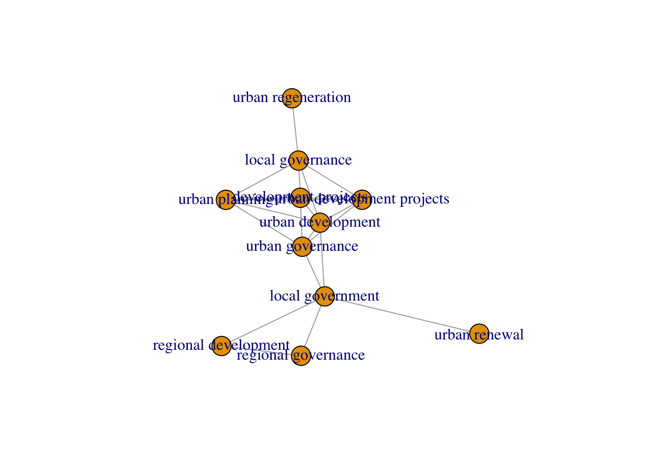
Identify the main keywords
search_terms <- litsearchr::get_keywords(reduced_graph)
head(sort(search_terms), 20)
[1] "development projects" "local governance"
[3] "local government" "regional development"
[5] "regional governance" "urban development"
[7] "urban development projects" "urban governance"
[9] "urban planning" "urban regeneration"
[11] "urban renewal" Identify isolated components of graph to suggest new keywords
components(reduced_graph)$membership
development projects local governance
1 1
local government regional development
1 1
regional governance urban development
1 1
urban development projects urban governance
1 1
urban planning urban regeneration
1 1
urban renewal
1
$csize
[1] 11
$no
[1] 1grouped <- split(names(V(reduced_graph)), components(reduced_graph)$membership)Write a new query based on additional keywords
litsearchr::write_search(grouped,
                         API_key = NULL,
                         languages = "English",
                         exactphrase = FALSE,
                         stemming = TRUE,
                         directory = "./",
                         writesearch = FALSE,
                         verbose = TRUE,
                         closure = "left")
[1] "English is written"[1] "(((develop* project*) OR (local* govern*) OR (region* develop*) OR (region* govern*) OR (urban* develop*) OR (urban* govern*) OR (urban* plan*) OR (urban* regener*) OR (urban* renew*)))"6 Drawing the PRISMA figure
Call the prisma() function to generate the PRISMA flowchart and replace the values with the actual counts from your study.
prismaplot <- prisma(
  found = nrow(all_references), # Total number of references found
  found_other = 0,               # Number of additional references found through other sources (if any)
  no_dupes = nrow(all_unique_references), # Number of unique references after removing duplicates
  screened = nrow(all_unique_references),  # Number of references screened
  screen_exclusions = 0,         # Number of references excluded during screening
  full_text = nrow(all_unique_references), # Number of references obtained in full text
  full_text_exclusions = 0,      # Number of references excluded during full-text assessment
  qualitative = nrow(all_unique_references), # Number of studies included in qualitative synthesis
  quantitative = nrow(all_unique_references), # Number of studies included in quantitative synthesis
  width = 800, height = 800  ,    # Specify width and height for the generated PRISMA flowchart
  font_size = 20
)

prismaplot
7 References
Van Marissing, E., Bolt, G., & Van Kempen, R. (2006). Urban governance and social cohesion: Effects of urban restructuring policies in two dutch cities. Cities, 23(4), 279–290. https://doi.org/doi.org/10.1016/j.cities.2005.11.001
Wu, F., & Zhang, F. (2022). Rethinking china’s urban governance: The role of the state in neighbourhoods, cities and regions. Progress in Human Geography, 46(3), 775–797. https://doi.org/doi.org/10.1177/03091325211062171